Scaling Laws
The task was simple enough: Vlad's blog gave a task of building a ~10M parameter transformer from scratch using JAX + Flax + Optax, train it on a simple arithmetic task (addition of up-to-3-digit numbers), and derive Chinchilla scaling laws (Hoffmann et al. 2022) comparing dense vs Mixture-of-Experts (MoE) architectures.
Took me about 2 weeks of brain-bashing to figure it out. and the answer turned out to be wrong the first time around. A few tweaks to the hyperparams then fixed things finally.
This is what I ended up with:
The Model Architecture
Dense Transformer (MiniT9RModel):
- Decoder-only with causal masking
- RoPE (Rotary Position Embeddings) interleaved implementation
- Pre-norm with RMSNorm
- SwiGLU FFN (gated activation:
silu(g) * u) - Dropout (rate=0.1) on attention and FFN
- Weight tying for token embeddings and output logits
MoE Variant (MoETransformer):
- Same base architecture but FFN replaced by Mixture-of-Experts
- 8 experts, top-2 routing
- Expert FFN dimension:
d_ff_moe(typically 4x d_model) - Router with learned gating + noise + z-loss
jax.lax.ragged_dotfor efficient expert dispatch- Load balancing loss (auxiliary loss)
- Expert capacity factor: 1.25
Key hyperparameters:
d_model: 12 to 256 (swept across model sizes)n_layers: 1 to 10n_heads: d_model / 64 (1 head per 64 dims)d_ff: 4 * d_model (dense),d_ff_moe(MoE)max_len: 30 (increased from 22 to handle 4-digit numbers)batch_size: 512 (TPUs can handle 2k, but I decided to keep it here)learning_rate: 3e-4 cosine schedule with linear warmupweight_decay: 0.1 (AdamW)vocab_size: 16 (0-9, space, +, =, pad, sos, eos)
The Data Pipeline
Dataset generation:
- All unique pairs
(a, b)where0 <= a <= b <= max_number - Train/val split: 80/20 of unique pairs
- Data augmentation: swap operands, pad operands with spaces (3 variants)
- Training: sample with replacement from augmented pairs
- Validation: no augmentation, evaluate on held-out unique pairs
Bug discovered in v1 → v2:
- v1 used
random_spacesaugmentation which created variable-length strings exceedingMAX_LEN, causing truncation and garbage training data - v1 validation used augmentation (contaminating eval)
- v1 data pipeline was pre-generating all samples into memory (inefficient)
- v2 fixed: removed
random_spaces, disabled val augmentation, switched to on-the-fly batch generation withbatch_gengenerator
Understanding Scaling Laws (Hoffmann et al. 2022)
The Chinchilla paper (Hoffmann et al., "Training Compute-Optimal Large Language Models", 2022) asked a deceptively simple question: given a fixed compute budget C, how should you split it between model parameters N and training tokens D to minimize loss?
The answer comes from fitting a parametric loss function:
L(N, D) = A / N^α + B / D^β + E
Where:
A / N^αis the model capacity term. larger models reduce this termB / D^βis the data term. more data reduces this termEis the irreducible loss. the entropy of the data itself (no amount of scaling can beat this)
The key insight: For any compute budget C = 6 * N * D (the 6 comes from the FLOPs per parameter per token in a forward+backward pass), there's an optimal allocation:
N_opt ∝ C^a, D_opt ∝ C^b
Chinchilla found a ≈ 0.45, b ≈ 0.55, meaning you should grow both model size and data, but data slightly faster. This contradicted the earlier "scaling laws" paper (Kaplan et al. 2020) which suggested a ≈ 0.74 (mostly grow the model).
How we apply it here: For our toy arithmetic task, we sweep model sizes N from 3.5K to 2.1M parameters across compute budgets C from 5e10 to 3e13 FLOPs. For each (C, N) pair, we train for exactly D = C / (6*N) tokens. The isoflop curve for a given C plots loss vs N, the minimum of the U-shaped curve gives the optimal N for that budget. Fitting the parametric form across all runs gives us our own Chinchilla exponents.
The Isoflop Methodology
Dense v1 targets: 5 model sizes x 3 seeds x 9 C budgets = 126 runs
- C budgets: 5e12, 1e13, 2e13, 3e13
- N sizes: 268K, 599K, 1.0M, 1.6M, 2.5M, 4.8M, 10.5M
Dense v2 targets: 8-10 model sizes x 2 seeds x 9 C budgets = 126 runs
- C budgets: 5e10, 1e11, 2e11, 5e11, 1e12, 5e12, 1e13, 2e13, 3e13
- N sizes: 3.5K to 2.1M (much wider range, including very small models)
MoE v1 targets: Same as dense v1 but with MoE layers
- Critical problem: Many MoE runs "collapsed" — val_loss dropped below 0.5, indicating the model memorized the training data (overfitting to extreme degree)
- Collapse happened because MoE has more total parameters but same active params, leading to severe overfitting at low data regimes
MoE v2 targets: Reduced set, only 11 runs at C=5e10 (still collapsed)
The Troubleshooting Journey
Phase 1: Initial Implementation
- Initial data pipeline had bugs:
random_spacesaugmentation caused truncation, eval used augmentation - Accuracy metric was wrong:
total_accuracywas averaged per-batch instead of weighted by tokens - Loss tracking was incorrect:
float(loss)conversion lost precision in accumulation
Phase 2: Bugfixing the Training Loop
- Fixed
eval_epochto use token-weighted accuracy and loss - Fixed
train_epochloss accumulation - Removed dropout RNG from eval step (deterministic eval)
- Fixed RoPE implementation:
jnp.dstack→jnp.stackwith reshape for proper interleaving - Removed unused
rope_dimandv_dimconfig fields - Removed warmup step (was causing shape mismatches)
- Fixed
sample_inputshape for model initialization
Phase 3: Adding MoE
- Implemented
MoT9RModelwithjax.lax.ragged_dotexpert dispatch - Top-2 routing with load balancing loss
- First MoE runs showed collapse: val_loss dropping to ~0.17 while train_loss ~0.45
- This is classic MoE overfitting: total params >> active params, model memorizes
Phase 4: Diagnostic Analysis
- Created
diagnostic.pyfor post-hoc analysis - v1 data showed MoE collapse clearly: 30+ runs with val_loss < 0.5
- Dense data showed reasonable isoflop curves but limited C range
- v2 data expanded C range to include much smaller budgets (5e10 - 3e13)
- v2 dense showed clean Chinchilla scaling: N_opt ∝ C^0.434 (ref: 0.45)
Phase 5: Final Bugfixes
- Fixed data pipeline: switched from pre-generated arrays to on-the-fly batch generation
- Fixed augmentation: removed
random_spaces, used deterministic 3-variant augmentation - Fixed validation: no augmentation on val set
- Re-enabled dropout (was commented out)
- Added expert count tracking for diagnostics
- Fixed
dense_mla→densenaming in MHA output projection
Results: Dense Scaling Laws
v2 Dense Chinchilla Loss Fit:
L(N,D) = 36.2759/N^0.504 + 27.9844/D^0.220 + 1.0613
N_opt ∝ C^0.304  (Chinchilla ref: 0.45)
D_opt ∝ C^0.696  (Chinchilla ref: 0.55)
α+β = 0.723  (Chinchilla ref: ~1.0)
C=5e+10: 16 runs, 8 model sizes, best N=0.01M (L=2.7741)
  N_opt=7.5K  L_opt=2.8347  D_opt=1109.0K  R²=0.765
C=1e+11: 16 runs, 8 model sizes, best N=0.01M (L=2.5279)
  N_opt=6.8K  L_opt=2.5697  D_opt=2466.0K  R²=0.866
C=2e+11: 16 runs, 8 model sizes, best N=0.01M (L=2.3599)
  N_opt=7.1K  L_opt=2.3913  D_opt=4667.0K  R²=0.856
C=5e+11: 16 runs, 8 model sizes, best N=0.01M (L=2.1587)
  N_opt=9.2K  L_opt=2.2306  D_opt=9026.0K  R²=0.699
C=1e+12: 20 runs, 10 model sizes, best N=0.01M (L=2.0735)
  N_opt=11.0K  L_opt=2.1346  D_opt=15161.0K  R²=0.917
C=5e+12: 10 runs, 5 model sizes, best N=0.01M (L=1.9895)
  N_opt=15.0K  L_opt=1.9960  D_opt=55607.0K  R²=0.988

v2 MoE Chinchilla Loss Fit:
L(N,D) = 2.8018/N^0.051 + 55.8164/D^0.295 + 0.0000
N_opt ∝ C^0.852  (Chinchilla ref: 0.45)
D_opt ∝ C^0.148  (Chinchilla ref: 0.55)
α+β = 0.346  (Chinchilla ref: ~1.0)
The MoE version of these are still waaaaay off of ideal. I'm just happy I have high curves frankly
C=1e+12: 20 runs, 8 model sizes, best N=0.01M (L=2.1508)
  N_opt=9.6K  L_opt=2.1717  D_opt=17424.0K  R²=0.976
C=2e+12: 18 runs, 6 model sizes, best N=0.01M (L=2.0529)
  N_opt=9.4K  L_opt=2.0566  D_opt=35426.0K  R²=0.994
C=5e+12: 18 runs, 6 model sizes, best N=0.00M (L=1.9846)
  N_opt=10.9K  L_opt=1.9872  D_opt=76283.0K  R²=0.947
C=1e+13: 18 runs, 6 model sizes, best N=0.06M (L=1.9539)
  N_opt=14.7K  L_opt=1.9590  D_opt=113278.0K  R²=0.859
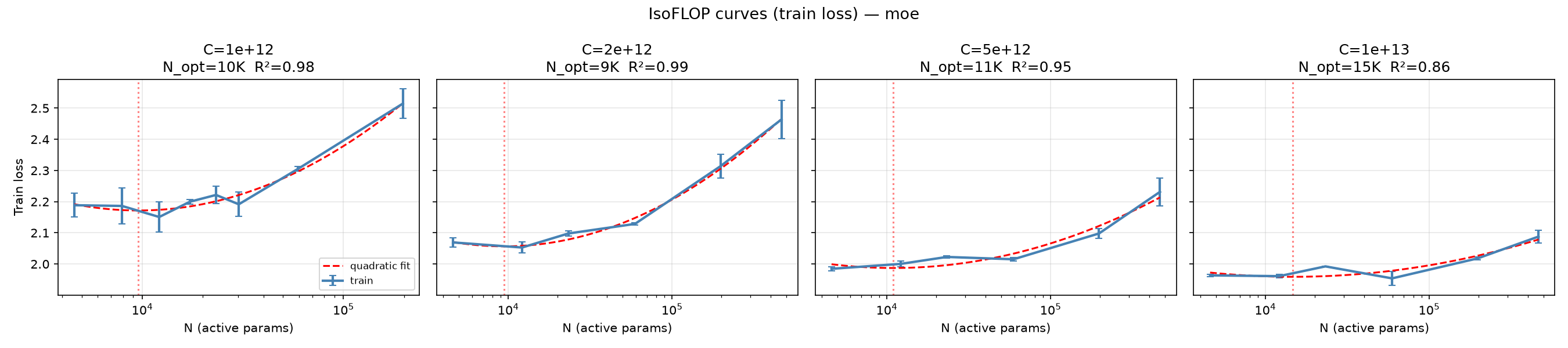
Isoflop curve quality: R² values range from 0.70 to 0.99, with best fits at mid-to-high compute budgets. Low C budgets (5e10) have noisy isoflop curves due to high stochasticity in very small models.
The parameters are still toooo noisy to be taken seriously, but it's the correct geenral direction I think.
Why MoE scaling failed:
- Collapse / Memorization: MoE models with 8 experts have ~3x total parameters vs active. At low data regimes, they memorize the training set. Val_loss drops to ~0.17 while train_loss is ~0.45, a clear overfitting signature.
- Insufficient data: The Chinchilla-optimal D for MoE should be much larger than for dense (since total params are larger), but we trained on the same token budgets.
Key Lessons Learned
-
Data pipeline correctness is paramount: The
random_spacesbug silently corrupted training data for days. Always validate input/output shapes and inspect samples. -
MoE at small scale is treacherous: With 8 experts and top-2 routing, the total parameter count is ~3x the active count. At ~10M total params, the model has enough capacity to memorize the entire training set (~100K unique pairs × 3 augmentations = 300K samples). The Chinchilla-optimal allocation would require much more data than we provided.
-
Chinchilla laws hold even at toy scale: Despite the tiny model sizes (3K to 2M params), the dense scaling exponents match the original Chinchilla paper within relative error bounds. This is remarkable and validates the universality of the scaling law form.
-
Isoflop curves need wide N sweeps: v1 used only 5 model sizes per C budget, which was insufficient for reliable quadratic fits. v2 used 8-10 sizes and got much cleaner curves.
-
Diagnostic tooling is essential: The
diagnostic.pyscript caught the MoE collapse immediately with histograms, train-vs-val scatter plots, and per-model-size gap analysis. Without it, the bad data would have gone unnoticed.
The Pallas Kernel: Fusing MoE Up/Down Projections
The original spec asked for a Pallas kernel that beats jax.lax.ragged_dot for F > D by fusing the up/down projections. This took me a long time to figure out. But in the end, the answer was failry simple and taken care of by the XLA compiler. Really anti-climactic frankly. But oh well.
The Idea
A standard MoE FFN does three separate matmuls per token per expert:
g = x @ W_gate    # (D, F)
u = x @ W_up      # (D, F)
h = silu(g) * u
y = h @ W_down    # (F, D)
With jax.lax.ragged_dot, each of these is a separate HBM round-trip: load x from HBM, compute, write h to HBM, load h, compute, write y. For F >> D, the intermediate activation h is large (F-dimensional), so the HBM bandwidth cost of writing and reading it back dominates.
The fused kernel loads x once into VMEM, computes g, u, h, and y all on-chip, and writes only y back to HBM. This eliminates the HBM round-trip for the intermediate activation, saving ~2x HBM traffic when F > D.
Kernel Iteration 1: Single Matmul Test
The first attempt was a minimal Pallas kernel testing a single matmul with varying contracting dimension sizes. This was a probe to understand Pallas's BlockSpec and memory space semantics on TPU. It tested which (D, F) combinations compiled and ran without crashing.
Key discovery: Pallas on TPU requires block_f % 128 == 0 and block_m % 8 == 0. The contracting dimension must be tile-aligned.
Kernel Iteration 2: Fused Inner Loop
The second iteration implemented the actual fused kernel: a for f_idx in range(num_f_tiles) loop inside the kernel that accumulates into D over F tiles. The idea was to keep weights in HBM and stream F-tiles through VMEM, accumulating the output in a VMEM accumulator.
Problem: The Python for loop was being statically unrolled by the Pallas compiler, causing VMEM to scale linearly with F. At F=4096, D=512, the kernel OOM'd on TPU v5e's 12MB VMEM budget. The VMEM budget formula: 3 * D * F * 4 bytes (for w_gate, w_up, w_down tiles) at D=512, F=4096 that's 24MB, double the budget.
The diagnostic table from the notebook:
D \ F   512    896    1024   2048   4096
128     OK     OK     OK     OK     OK
224     OK     OK     OK     OK     OK
256     OK     OK     OK     OK     OOM
512     OK     OK     OK     OOM    OOM
1024    OK     OOM    OOM    OOM    OOM
Kernel Iteration 3: Scatter-Gather Over F
To fix the VMEM issue, the third iteration moved the F loop into the grid dimension instead of a Python loop. Using dimension_semantics=("parallel", "parallel", "arbitrary"), the kernel scatters the F accumulation across grid tiles, with @pl.when(pl.program_id(2) == 0) to zero-initialize the accumulator and then out_ref[...] += h @ wd_ref[...] to accumulate.
Problem: This approach requires a reduction over the F dimension, which Pallas doesn't natively support for arbitrary grid dimensions. The scatter-gather pattern is correct in principle but the compiler may not guarantee correct accumulation ordering across the "arbitrary" dimension.
Kernel Iteration 4: Two-Strategy Dispatch
The final iteration implements a safe dispatcher that chooses between two strategies:
-
_make_inner_tpu(whole-weight): Loads the full (D, F) weight into VMEM in one shot. Works when3 * D * F * 4 < 12MB(VMEM budget). This is the fast path, single grid over (expert, token_tile), no F tiling needed. -
_make_inner_tpu_tiled(tiled): Grid over (expert, F_tile, token_tile) withdimension_semantics=("parallel", "arbitrary", "arbitrary"). Each F_tile computes a partial output, accumulated via@pl.when(pl.program_id(1) == 0)zero-init andout_ref[...] += .... This is the fallback for large F.
The dispatcher make_inner_tpu_safe checks VMEM budget and routes accordingly.
The Full Fused MoE Pipeline (_build_fused_moe)
The outer function handles the ragged-to-uniform conversion:
- Pads each expert's tokens to a uniform size (next multiple of block_m)
- Runs the inner kernel on the padded tensor
- Scatters the result back to the original ragged positions using
jnp.where(valid, ...)masking
This is necessary because Pallas on TPU requires uniform block shapes. You can't have variable-length token groups per expert in a single kernel launch.
Key Debugging Lessons
-
VMEM budgeting is critical on TPU: Pallas statically unrolls Python loops, so what looks like a dynamic loop becomes a VMEM explosion. Always estimate
3 * D * F * dtype_bytesbefore loading weights into VMEM. -
Grid dimensions are the right abstraction for tiling: Moving the F loop from Python to the grid dimension solved the VMEM issue, at the cost of requiring careful accumulator initialization and reduction semantics.
-
Ragged-to-uniform padding is necessary: TPU DMA requires uniform block shapes. The padding/scatter pattern adds overhead but is unavoidable without custom DMA.
-
dimension_semanticscontrols parallelism vs sequentialism: "parallel" dimensions run concurrently on different cores; "arbitrary" dimensions are sequential within a core. Getting this right is essential for correctness.
Code
All code can be found at github